The Investment Wisdom in Kelly Criterion

In 1956, John L. Kelly, Jr. proposed the famous Kelly criterion while working at Bell Labs. He pointed out that the mathematical model used by Claude Shannon in the theory of communication noise interference is also applicable to investors’ risk and return management.

Kelly’s paper was a sensation as soon as it was published, and many mathematical geniuses carried it forward in gambling or investment and made extraordinary achievements. Edward Thorp, who discovered loopholes in blackjack, applied the Kelly criterion to manage funds and beat US casinos. At the same time, Warren Buffett successfully applied the Kelly criterion in his investment portfolio.

Let us first take a look at this magical formula:

Here, f* is the proportion of capital that should be invested in each transaction; p represents the probability of making money in each transaction, that is, the probability of a win; b represents the profit corresponding to each unit loss, that is, the odds (profit-to-loss ratio); q represents the probability of losing money for each transaction, that is, q=1-p.

The numerator in the Kelly criterion represents the expected net winnings per unit bet. Therefore,

(1) When the expected net winnings (bp-q) = 0, it is a fair game, and no bets should be placed;

(2) When the expected net winnings (bp-q)<0, there is no advantage, and no bets should be placed either;

(3) When the expected net winnings (bp-q)>0, then investing according to the Kelly criterion maximizes return while minimizing risk.

In fact, the Kelly criterion tells us how to allocate investment proportions reasonably with minimal risk. Only by increasing capital on assets with high winning rate and high odds, reducing capital on assets with low winning rate and low odds, and continuously adjusting the proportion according to market dynamics, can we generate a continuous and steady return.

To successfully apply the Kelly criterion to an asset investment, we first need to form a reasonable expectation of the corresponding winning rate and odds. The winning rate of an asset investment depends on its fundamentals: the faster the asset appreciates in value, the higher its corresponding winning rate. In contrast, the odds of an asset investment are determined by the market: the higher the short-term trading sentiment for an asset, the higher its price, and the lower its investment odds become.

Panoramic Industry Analysis

Datayes! recently introduced the “Panoramic Industry Analysis” feature. Leveraging the wisdom in the Kelly criterion, the new feature provides a comprehensive and multi-dimensional analysis on the cost performance of various industries by evaluating metrics such as industry prosperity, market trends, valuations and congestion.

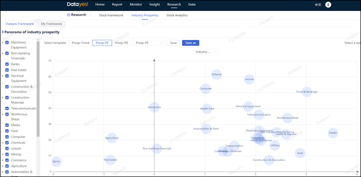
Figure 1. A screenshot of the Panoramic Industry Analysis feature

Industry Prosperity reflects the dynamic changes in fundamentals of corresponding industries.  Market Trend Intensity reflects the market’s reaction to changes in industry fundamentals. Together, these metrics describe the winning rate of an industry.

Industry valuation and trade congestion show how much the market has priced-in on industry fundamentals; as such, these metrics describe the odds. The Panoramic Industry Analysis uses these metrics to offer investors a comprehensive and essential tool in selecting industries and allocation.

Industry Prosperity

Datayes! developed industry fundamental analysis frameworks based on the “fundamental + quantitative” paradigm, that takes macro and industry chains with uses artificial intelligence to perform Nowcast on industry prosperity. Compared to the corresponding proxy metric, the industry prosperity score achieved an 87% winning rate in forecasting directional change during Q4 2020 to Q1 2021, that had a long gap without official announcements.

The industry prosperity score is a daily forecast on fundamental values based on high frequency macro and industry data, and is more sensitive to marginal changes of industry fundamental drivers. While short-term movements in industry indices are not entirely determined by fundamental changes, a continuous positive fundamental valuation is a core driving factor for long-term performance.

Let’s take the non-ferrous metal industry as an example. In March 2020, with the recovery of demand brought by the resumption of work and production, the industry’s prosperity rebounded in April and reached a three-year high in August. Subsequently, the industry’s fundamentals remained relatively stable until the end of 2020 to Q1 of 2021 when the full recovery of major economies and the rebound in global demand fueled a continuous rise in commodity prices. Similarly, the market confirmed the rise in prosperity and reflected this in the periods of May-June and October-December.

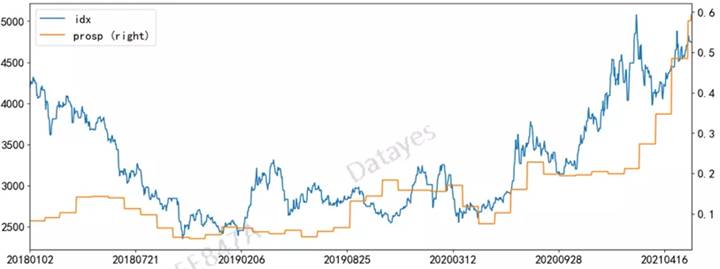
Figure 2. Prosperity of the non-ferrous metal industry (Blue: industry index; Orange: monthly prosperity index)

Market Trend

Tracking market trends is a classic investment strategy.  Assets with recent positive returns may continue the trend for a period in the future.  On the other hand, when the market trend intensity is high, there is risk of trend reversal.

By computing market trend intensity, we can effectively reduce the time cost of holding assets, and combined with timely judgement of excessive market trend intensity, we can realize portfolio returns while reducing risk to volatility.

The non-ferrous metal industry sample shows us that the trend signal roughly reflects the mid-to-long-term trend of the industry index, and when the trend intensity exceeds twice the standard deviation, the industry index tends to pull back. In Q3 of 2020 and Q1 of 2021, the non-ferrous metal industry had undergone a relatively large degree of adjustments, and the industry trend intensity returned close to the average line.

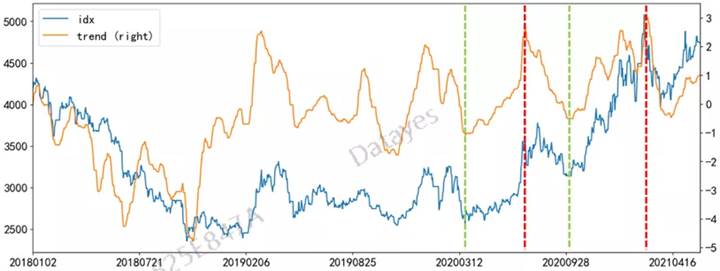
Figure 3. Market trend intensity of the non-ferrous metal industry (Blue: industry index; Orange: market trend intensity)

Industry Valuation

In the long run, asset prices resolve around their corresponding fundamental valuation. Commonly used fundamental valuation metrics include Price-to-Earnings (PE) ratio and Price-to-Book (PB) ratio. Generally, industries with low valuation multiples are more cost-effective than industries with high valuation multiples. However, certain industries such as banks and real estate have had historically low valuations while growth industries such as technology and medicine generally have high valuations. Therefore, we calculate quantiles of the current PE/PB against historical values to better compare price/valuation ratios of different industries horizontally.

Taking the non-ferrous metal industry as an example, the PE quantile of the industry in August 2020 and February 2021 were at 3-year highs, and as observed subsequently, the index began to decline under pressure.

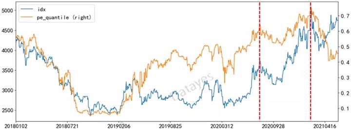
Figure 4. Non-ferrous metal industry valuation analysis (Blue: industry index; Orange: PE historical quantile)

Market Congestion

Irrational trades in a market brings short term volatility to asset prices. Sharp rises in price and volume and sudden increase in volatility are indications that the market is overheating and there is excessive trading congestion. The higher the congestion, the higher the risk of a future market crash is. We first characterize the degree of congestion from the perspectives of liquidity and deviation of volume and price, and then combine multiple measures into a unified market congestion measure.

Going back to the non-ferrous metals industry, we observed that in August 2020 and February 2021, the turnover ratio of the industry was high while price and volume trends started to diverge. It proved to be an early risk warning consequent to the sharp decline in industry index.

Liquidity

Liquidity is commonly measured using volume, turnover and turnover ratio. High trading volume and turnover ratio mean that an industry is over congested, overdrawing future liquidity, and there is a downside risk. We calculate liquidity by dividing an industry’s trade volume by the industry’s outstanding shares over a period of time.

Volume-Price Divergence

Under normal circumstances, changes in asset liquidity and asset price follow the same trends and when there is a divergence, it is an indication that the price trend will reverse. For example, if the stock price increases, but the trading volume decreases, there is a lack of subsequent upward momentum and the trend is unsustainable. In addition, if the trade volume is high, but the stock price does not continue to rally, it indicates a divergence between long and short trades, and consequently, there is downside risk. We use the correlation between the industry index and industry trade volume over a period to describe the degree of volume-price divergence. The negative sign in the formula ensures that a high value of this indicator denotes a high degree of volume-price divergence.

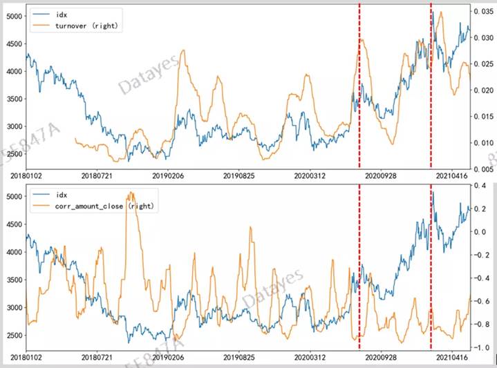
Figure 5. Market congestion of the non-ferrous metal industry (Blue: industry index; Orange: market congestion)

Industry Investment Value Comparison

The metrics discussed earlier describe the cost performance of individual industries from different angles. To perform a horizontal industry comparison on corresponding cost performances, we would need to put together various metrics for a comprehensive comparison and analysis. We take the market as of the end of May 2021 as an example to illustrate the practical application of the panoramic industry analysis graph.

Prosperity and Market Trend

Due to low base figures last year caused by the COVID-19 pandemic, most industries show relatively higher prosperities this year, judging from the corresponding prosperity scores and their marginal changes. However, apart from mining, chemical, construction materials, and steel, which are enjoying their pricing power as upstream in the economic cycle, most industries began to weaken marginally.

Correspondingly, from the perspective of the industry prosperity and market trend intensity, the market has continuously adjusted since March to reflect changes in fundamental valuation. Currently, the trend intensity of most industry indices has peaked, and the industries face risk to crash as fundamental valuations continue to weaken.

On the contrary, the current fundamental prosperity of banking, non-banking financial and electronics industries are at relative lows, while their fundamentals show continuous improvement. Recently, the intensity of market trends in these industries has gradually increased, reflecting the market’s continuous pricing changes in accordance to the industry fundamentals, and showing that investment in these industries have a relatively good winning rate.

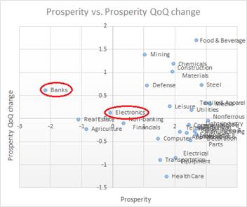
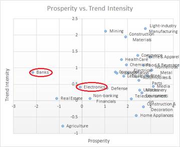
Figure 6: Scatter plot showing industry prosperity vs. its QoQ change (left), and industry prosperity vs. trend intensity (right)

Valuation and Congestion

From the scatter plot showing trend intensity and valuation, we can see that the automotive, food and beverage, and pharmaceuticals and biomedical industries have high trend intensity and valuations.  Meanwhile, from the trend intensity and congestion scatter plot, industries such as steel, non-ferrous metals, and food and beverage have high trend intensity and high congestion, requiring continuous monitoring of the impact of market preference on corresponding industries.

In contrast, industries such as banking, non-banking finance, and electronics all have positive fundamentals while having relatively lower valuation and congestion, which also means that investing in these industries now would have higher odds.

By performing a comprehensive analysis using metrics that reflect industry winning rates and the odds, we can obtain the most cost-effective industry allocation.

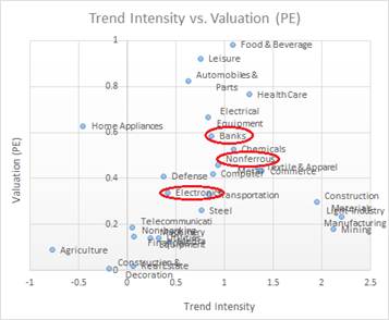
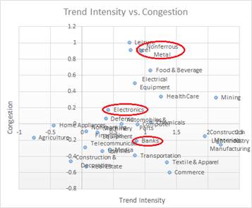
Figure 7: Industry index trend intensity, valuations and congestion